Pandas rolling(): Moving Averages and Time Windows
Use rolling() to summarize a moving set of observations. Choose a fixed row count or a time interval, decide how many known values are required, and apply an aggregation such as mean() or sum().

Calculate a two-row rolling sum 🔝
rolling() creates a window object; call sum(), mean() or another aggregation to obtain values. The first row is missing because the default for an integer window requires that many known observations.
import pandas as pd
import numpy as np

def student_data():
    return pd.DataFrame({"name": ["Alex", "King", "Ravi", "Raju", "John"], "mark": [7, 8, 5, 6, 3]})

df = student_data()
df["my_sum"] = df["mark"].rolling(2).sum()
print(df)
assert df["my_sum"].iloc[1:].tolist() == [15, 13, 11, 9]
Expected output
   name  mark  my_sum
0  Alex     7     NaN
1  King     8    15.0
2  Ravi     5    13.0
3  Raju     6    11.0
4  John     3     9.0
Allow partial windows with min_periods 🔝
min_periods=1 permits a result with one known observation. It does not change the maximum window size of two. For integer windows the default minimum is the window size; for time-offset windows it is one.
df = student_data()
df["my_sum"] = df["mark"].rolling(2, min_periods=1).sum()
print(df)
assert df["my_sum"].tolist() == [7, 15, 13, 11, 9]
Expected output
   name  mark  my_sum
0  Alex     7     7.0
1  King     8    15.0
2  Ravi     5    13.0
3  Raju     6    11.0
4  John     3     9.0
Calculate a moving average 🔝
Select the numeric measure explicitly. The rolling mean of adjacent marks is 7.5, 6.5, 5.5 and 4.5. Student order is only a practice sequence here; a moving average of unrelated students does not represent a time trend.
df = student_data()
df["moving_mean"] = df["mark"].rolling(2).mean()
print(df)
assert df["moving_mean"].iloc[1:].tolist() == [7.5, 6.5, 5.5, 4.5]
Expected output
   name  mark  moving_mean
0  Alex     7          NaN
1  King     8          7.5
2  Ravi     5          6.5
3  Raju     6          5.5
4  John     3          4.5
Roll across numeric columns with transpose 🔝
Current Pandas rolling() has no axis argument. To roll across columns, select numeric fields, transpose, roll and transpose back. Column order defines the sequence, so this is meaningful only for compatible ordered measures.
df = student_data()
df["math"] = [70, 80, 50, 60, 30]
result = df[["mark", "math"]].T.rolling(2).sum().T
print(result)
assert result["math"].tolist() == [77, 88, 55, 66, 33]
Expected output
   mark  math
0   NaN  77.0
1   NaN  88.0
2   NaN  55.0
3   NaN  66.0
4   NaN  33.0
Avoid aggregating unrelated text columns 🔝
Select the intended numeric Series before rolling. A mixed table can raise a DataError when a text column is included in a numeric aggregation. See dtypes.
df = student_data()
df["class1"] = ["One", "Two", "Three", "Four", "Five"]
df["math"] = [70, 80, 50, 60, 3]
df["my_sum"] = df["math"].rolling(2).sum()
print(df)
assert df["my_sum"].iloc[1:].tolist() == [150, 130, 110, 63]
Expected output
   name  mark class1  math  my_sum
0  Alex     7    One    70     NaN
1  King     8    Two    80   150.0
2  Ravi     5  Three    50   130.0
3  Raju     6   Four    60   110.0
4  John     3   Five     3    63.0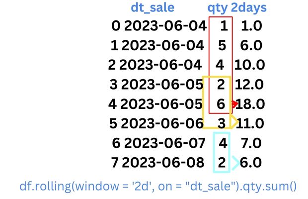
Use a two-day time window with on 🔝
Parse and sort timestamps before time-based rolling. on identifies the time column; it is not the measure being averaged. The default closed="right" includes the current timestamp and excludes the exact left boundary. Multiple rows on one date accumulate in their current order.
sales = pd.DataFrame({
    "dt_sale": ["2023-06-04", "2023-06-04", "2023-06-04", "2023-06-05", "2023-06-05", "2023-06-06", "2023-06-07", "2023-06-08"],
    "qty": [1, 5, 4, 2, 6, 3, 4, 2]
})
sales["dt_sale"] = pd.to_datetime(sales["dt_sale"], format="%Y-%m-%d")
sales = sales.sort_values("dt_sale", kind="stable")
sales["2days"] = sales.rolling("2D", on="dt_sale")["qty"].sum()
print(sales)
assert sales["2days"].tolist() == [1, 6, 10, 12, 18, 11, 7, 6]
Expected output
     dt_sale  qty  2days
0 2023-06-04    1    1.0
1 2023-06-04    5    6.0
2 2023-06-04    4   10.0
3 2023-06-05    2   12.0
4 2023-06-05    6   18.0
5 2023-06-06    3   11.0
6 2023-06-07    4    7.0
7 2023-06-08    2    6.0
Compare windows based on two date columns 🔝
The same quantities can fall into different windows under sale and purchase timestamps. Each time column must be monotonic for its calculation. In this sample both are already ordered; if their sort orders differ, calculate separately and realign by a stable row identifier.
table = pd.DataFrame({
    "dt_sale": ["2023-06-04", "2023-06-04", "2023-06-04", "2023-06-05", "2023-06-05", "2023-06-06", "2023-06-08", "2023-06-08"],
    "dt_buy": ["2023-06-03", "2023-06-04", "2023-06-04", "2023-06-05", "2023-06-05", "2023-06-06", "2023-06-07", "2023-06-08"],
    "qty": [1, 5, 4, 2, 6, 3, 4, 2]
})
for column in ["dt_sale", "dt_buy"]:
    table[column] = pd.to_datetime(table[column], format="%Y-%m-%d")
    assert table[column].is_monotonic_increasing
table["2d_sale"] = table.rolling("2D", on="dt_sale")["qty"].sum()
table["2d_buy"] = table.rolling("2D", on="dt_buy")["qty"].sum()
print(table)
assert table["2d_buy"].tolist() == [1, 6, 10, 11, 17, 11, 7, 6]
Expected output
     dt_sale     dt_buy  qty  2d_sale  2d_buy
0 2023-06-04 2023-06-03    1      1.0     1.0
1 2023-06-04 2023-06-04    5      6.0     6.0
2 2023-06-04 2023-06-04    4     10.0    10.0
3 2023-06-05 2023-06-05    2     12.0    11.0
4 2023-06-05 2023-06-05    6     18.0    17.0
5 2023-06-06 2023-06-06    3     11.0    11.0
6 2023-06-08 2023-06-07    4      4.0     7.0
7 2023-06-08 2023-06-08    2      6.0     6.0
Distinguish two observations from two days 🔝
With irregular timestamps, rolling(2) always uses adjacent observations, while rolling("2D") uses the time interval. A time window does not generate missing dates or fill gaps.
events = pd.DataFrame({"date": pd.to_datetime(["2026-01-01", "2026-01-02", "2026-01-10"]), "amount": [10, 20, 30]})
events["two_rows"] = events["amount"].rolling(2, min_periods=1).sum()
events["two_days"] = events.rolling("2D", on="date")["amount"].sum()
print(events)
assert events.loc[2, "two_rows"] == 50
assert events.loc[2, "two_days"] == 30
Expected output
        date  amount  two_rows  two_days
0 2026-01-01      10      10.0      10.0
1 2026-01-02      20      30.0      30.0
2 2026-01-10      30      50.0      30.0
Control the time-window boundaries with closed 🔝
For a trailing two-day interval, right includes the current time but not the left boundary; left excludes the current time but includes the left boundary; both includes both; neither excludes both. The first result can be missing when no observations remain.
values = pd.Series([10, 20, 30], index=pd.date_range("2026-01-01", periods=3, freq="D"))
result = pd.DataFrame({mode: values.rolling("2D", closed=mode).sum() for mode in ["right", "left", "both", "neither"]})
print(result)
assert result.iloc[2]["right"] == 50
assert result.iloc[2]["both"] == 60
Expected output
            right  left  both  neither
2026-01-01   10.0   NaN  10.0      NaN
2026-01-02   30.0  10.0  30.0     10.0
2026-01-03   50.0  30.0  60.0     20.0
Require enough known observations in each window 🔝
Missing entries do not satisfy min_periods. A three-row window with one missing value can still produce a subtotal with min_periods=2. Filling unknown sales with zero would change their meaning; see fillna().
values = pd.Series([10, np.nan, 30, 40])
print(pd.DataFrame({"value": values, "require_three": values.rolling(3).sum(), "require_two": values.rolling(3, min_periods=2).sum()}))
assert values.rolling(3, min_periods=2).sum().iloc[2] == 40
assert pd.isna(values.rolling(3).sum().iloc[2])
Expected output
   value  require_three  require_two
0   10.0            NaN          NaN
1    NaN            NaN          NaN
2   30.0            NaN         40.0
3   40.0            NaN         70.0
Compare trailing and centered windows 🔝
center=True labels windows at their center. Centered windows can incorporate later observations, so do not use them as historical predictors available at the label time. For a trailing feature excluding the current observation, shift the measure before rolling.
values = pd.Series([10, 20, 30, 40, 50])
result = pd.DataFrame({"value": values, "trailing": values.rolling(3).mean(), "centered": values.rolling(3, center=True).mean(), "prior_only": values.shift(1).rolling(3).mean()})
print(result)
assert result.loc[1, "centered"] == 20
assert result.loc[3, "prior_only"] == 20
Expected output
   value  trailing  centered  prior_only
0     10       NaN       NaN         NaN
1     20       NaN      20.0         NaN
2     30      20.0      30.0         NaN
3     40      30.0      40.0        20.0
4     50      40.0       NaN        30.0
Evaluate integer windows at a chosen step 🔝
step=2 evaluates every second result position, reducing output length. Use an integer window; time-offset rolling does not support step in the same way.
values = pd.Series([1, 2, 3, 4, 5, 6])
result = values.rolling(3, min_periods=1, step=2).sum()
print(result)
assert result.index.tolist() == [0, 2, 4]
assert result.tolist() == [1, 6, 12]
Expected output
0     1.0
2     6.0
4    12.0
dtype: float64
Calculate several rolling statistics 🔝
agg() returns several summaries of the same windows. std() defaults to a sample standard deviation with ddof=1; specify ddof=0 separately for a population-style calculation. Prefer built-in aggregations to custom Python functions when possible.
values = pd.Series([10, 20, 30, 40])
print(values.rolling(3).agg(["sum", "mean", "min", "max", "count"]))
print("Population standard deviation:")
print(values.rolling(3).std(ddof=0))
Expected output
    sum  mean   min   max  count
0   NaN   NaN   NaN   NaN    NaN
1   NaN   NaN   NaN   NaN    NaN
2  60.0  20.0  10.0  30.0    3.0
3  90.0  30.0  20.0  40.0    3.0
Population standard deviation:
0         NaN
1         NaN
2    8.164966
3    8.164966
dtype: float64
Practical workflow: aggregate daily sales before smoothing 🔝
A rolling average of transactions differs from an average of daily totals. Aggregate first when the question concerns daily performance. This synthetic extract covers every day in the reporting interval; missing days in real data need a justified policy. Explore resample().
transactions = pd.DataFrame({"date": pd.to_datetime(["2026-01-01", "2026-01-01", "2026-01-02", "2026-01-03", "2026-01-04"]), "amount": [10, 5, 20, 30, 40]})
daily = transactions.set_index("date")["amount"].resample("D").sum(min_count=1)
report = daily.rename("daily_sales").to_frame()
report["three_day_mean"] = daily.rolling(3, min_periods=3).mean()
print(report)
assert np.isclose(report["three_day_mean"].iloc[2], 65 / 3)
# Optional export in Colab:
# report.to_csv("daily_sales_trend.csv")
Expected output
            daily_sales  three_day_mean
date
2026-01-01           15             NaN
2026-01-02           20             NaN
2026-01-03           30       21.666667
2026-01-04           40       30.000000
Keep product histories separate 🔝
Group before rolling so one product does not affect another product’s moving average. Sorting defines the sequence within each product. transform returns a Series aligned with the source rows.
products = pd.DataFrame({"product": ["Pen", "Book", "Pen", "Book"], "date": pd.to_datetime(["2026-01-01", "2026-01-01", "2026-01-02", "2026-01-02"]), "sales": [10, 100, 20, 200]})
products = products.sort_values(["product", "date"], kind="stable")
products["moving_mean"] = products.groupby("product")["sales"].transform(lambda group: group.rolling(2, min_periods=1).mean())
print(products)
assert products.loc[2, "moving_mean"] == 15
assert products.loc[3, "moving_mean"] == 150
Expected output
  product       date  sales  moving_mean
1    Book 2026-01-01    100        100.0
3    Book 2026-01-02    200        150.0
0     Pen 2026-01-01     10         10.0
2     Pen 2026-01-02     20         15.0
Additional window options 🔝
win_type uses a supported SciPy window and requires SciPy; some window types need extra aggregation arguments. The default equal weighting needs no SciPy window. method="table" is intended for table-wide execution with engine="numba" in supported aggregations, not ordinary mixed-column averaging. Custom BaseIndexer windows are an advanced option. Start with the basic window and verify its meaning before adding complexity.
Common questions and pitfalls 🔝
Why are early results missing? The window has fewer known observations than min_periods. Why does a two-day window contain more than two rows? It includes all observations in the time interval. Why does axis fail? Use numeric_table.T.rolling(...).aggregation().T in current Pandas. Why does on fail? Check datetime parsing, missing timestamps and monotonic order. Why do centered features use future data? Their windows extend around the label. How do I create a trend chart? Plot the daily totals and moving average with line charts.
Exercise: compute a trailing three-day average 🔝
Create daily amounts 10, 20, 30 and 40 on four consecutive dates. Require all three observations in each moving average. Then calculate a prior-only average that excludes the current day. Expect trailing averages 20 and 30 at days three and four; the prior-only average at day four is 20.
Exercise solution 🔝
shift(1) makes the input at each date the previous day’s value before the trailing window is applied.
amounts = pd.Series([10, 20, 30, 40], index=pd.date_range("2026-01-01", periods=4, freq="D"))
answer = pd.DataFrame({"amount": amounts, "trailing": amounts.rolling(3).mean(), "prior_only": amounts.shift(1).rolling(3).mean()})
print(answer)
assert answer["trailing"].iloc[2:].tolist() == [20, 30]
assert answer["prior_only"].iloc[3] == 20
Expected output
            amount  trailing  prior_only
2026-01-01      10       NaN         NaN
2026-01-02      20       NaN         NaN
2026-01-03      30      20.0         NaN
2026-01-04      40      30.0        20.0
Practice in Google Colab 🔝
Open in Google Colab View on GitHub
Run the examples in order, change window sizes and missing values, then compare the moving totals and averages. Save your own copy to keep edits. All sample tables are included in the notebook.
Continue with data exploration and analysis, mean(), sum(), max() and std().
Reference: Pandas DataFrame.rolling documentation.

Subhendu Mohapatra
Author & Instructor at plus2net
I write and maintain practical tutorials on Python, PHP, SQL, JavaScript, HTML, jQuery, and web development at plus2net. The tutorials focus on clear explanations, working examples, and code that readers can test and adapt while learning.


Subscribe to our YouTube Channel here

 Python Video Tutorials