Pandas: Python Data Analysis and Manipulation Guide
Core Purpose & Overview
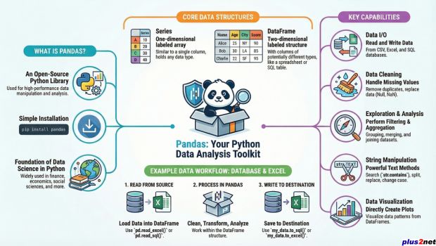
Pandas is Python's premier open-source library engineered for fast, flexible, and intuitive data manipulation and analysis on structured tabular data. It bridges the gap between raw data storage (spreadsheets, SQL databases, CSVs, JSON) and downstream analytical processing (statistics, machine learning, and visualization) through two primary labeled data structures: Series (one-dimensional) and DataFrames (two-dimensional).
Primary Use Cases: Automated ETL pipelines, data wrangling and cleaning, statistical aggregations via SQL-like groupby(), time-series analysis, and cross-format data interchange.
What Pandas Can Do & Where It Is Used 🔝
Pandas empowers developers, data analysts, and researchers to execute complex data wrangling workflows in minimal lines of readable Python. Key capabilities include:
- Data Ingestion & Serialization: High-speed parsers for CSV, Excel, JSON, Parquet, and relational SQL engines.
- Intelligent Alignment: Automatic label-based indexing that aligns mismatched datasets during arithmetic operations.
- Missing Data Imputation: Flexible tools to identify, fill, or drop null and NaN values across rows or columns.
- Reshaping & Pivoting: Powerful multi-dimensional pivot tables, melting, stacking, and hierarchical grouping.
- High-Performance Aggregations: Split-apply-combine paradigms that aggregate large datasets by categories in milliseconds.
Pandas is ubiquitously adopted in quantitative finance, business intelligence, healthcare data modeling, machine learning feature engineering, and scientific research. It integrates seamlessly with scientific Python libraries including NumPy for numerical computations, Matplotlib for plotting, and Scikit-learn for statistical modeling.
Installing, Checking Version & Upgrading 🔝
Install Pandas using the Python package manager (pip) in your terminal or virtual environment:
# Install standard Pandas library
pip install pandas

# Upgrade an existing installation to the latest stable release
pip install --upgrade pandas
Verify your installation and inspect the active version in Python:
import pandas as pd

print("Pandas Version :", pd.__version__)
Sample Output:
Pandas Version : 2.2.3Core Data Structures: Series vs. DataFrame 🔝
Pandas provides two foundational data structures designed for one-dimensional and two-dimensional data respectively:
1. Pandas Series (1D)
A one-dimensional labeled array capable of holding any data type (integers, strings, floating-point numbers, Python objects). It consists of an array of data values aligned with an explicit index array.
Explore Pandas Series →2. Pandas DataFrame (2D)
A two-dimensional labeled tabular structure with rows and columns of potentially heterogeneous data types. Think of a DataFrame as a spreadsheet or an in-memory SQL table composed of aligned Series columns.
Explore Pandas DataFrame →Here is how to create both structures in Python:
import pandas as pd

# 1. Create a 1D Pandas Series with custom day labels
temperatures = pd.Series([28.5, 31.0, 26.2, 29.8], index=["Mon", "Tue", "Wed", "Thu"], name="Temp_C")
print("--- Pandas Series ---")
print(temperatures)
print("Average Temp:", temperatures.mean())

# 2. Create a 2D Pandas DataFrame from a dictionary of lists
student_data = {
    "id": [1, 2, 3, 4],
    "name": ["Ravi", "Raju", "Alex", "Sophia"],
    "math": [85, 72, 91, 78],
    "english": [78, 88, 85, 92]
}
df_students = pd.DataFrame(student_data)
print("
--- Pandas DataFrame ---")
print(df_students)
Output:
--- Pandas Series ---
Mon    28.5
Tue    31.0
Wed    26.2
Thu    29.8
Name: Temp_C, dtype: float64
Average Temp: 28.875

--- Pandas DataFrame ---
   id    name  math  english
0   1    Ravi    85       78
1   2    Raju    72       88
2   3    Alex    91       85
3   4  Sophia    78       92
To inspect structural properties and available operations on DataFrames, see DataFrame Attributes → and DataFrame Methods →.
Five Essential Diagnostic Functions 🔝
When loading any new dataset into Pandas, five diagnostic methods and attributes provide an instant health check of your data structure and memory schema:
| Diagnostic Tool | Syntax / Type | Description & Purpose |
|---|---|---|
head(n) | Method | Returns the first n rows (default 5) for quick visual verification. |
tail(n) | Method | Returns the last n rows (default 5) to inspect end-of-file rows and total scope. |
shape | Attribute | Returns a tuple (rows, columns) representing the matrix dimensions. |
columns | Attribute | Returns the list of column header labels along axis 1. |
info() | Method | Prints index type, column names, non-null counts, dtypes, and memory usage. |
Video Tutorial: Five Important Basic Pandas DataFrame Functions
Practice using data from our Sample Student DataFrame tutorial.The code below demonstrates these five diagnostic methods in action:
import pandas as pd

# Diagnostic inspection on DataFrame
print("First 2 rows (head):
", df_students.head(2))
print("
Last 2 rows (tail):
", df_students.tail(2))
print("
Matrix Shape (rows, columns):", df_students.shape)
print("Column Names:", list(df_students.columns))

print("
Technical Summary (info):")
df_students.info()
Data Exploration, Analysis & Cleaning Modules 🔝
Modern data workflows require rigorous exploratory data analysis (EDA) and data cleansing before modeling:
Data Exploration & Analysis
Calculate statistical summaries (describe()), aggregate metrics using groupby(), filter row subsets, and merge disparate tables.
Data Cleaning & Imputation
Handle missing NaN records (fillna(), dropna()), deduplicate rows (drop_duplicates()), and cast types (astype()).
Explore specialized data operations:
- Creating DataFrames from NumPy Arrays — Convert multidimensional NumPy matrices into labeled tabular DataFrames.
- Email Validation with Pandas — Validate and cleanse email address formats across tabular columns using regular expressions.
- DataFrame Styling & Formatting — Apply CSS highlight colors, currency formatting, and conditional bar charts directly in Jupyter and HTML outputs.
- Pandas Date & Time Guide — Master timestamps, frequency resampling, date offsets, and time-series indexing.
Comprehensive Practice Exercises 🔝
Solidify your understanding by solving real-world challenges across our curated exercise tracks:
| Exercise Guide | Core Topics Covered | Action |
|---|---|---|
| Exercise 1 | Basic data handling, DataFrame construction, and row/column selection | Solve Exercise → |
| Exercise 1-1 | Binning with cut(), categorical grouping, and graph visualization | Solve Exercise → |
| Exercise Advanced | Multi-table merge(), join types, and complex groupby() operations | Solve Exercise → |
| Exercise 2 | String matching with str.contains(), aggregations (max(), min(), len()) | Solve Exercise → |
| Exercise 3 | Date-time operations combined with group-level aggregations | Solve Exercise → |
| Exercise 3-2 | Date component extraction (day, month, year) and datetime conversion | Solve Exercise → |
| Exercise 3-3 | Time-series grouping on backlink logs and SEO traffic analytics | Solve Exercise → |
| Exercise 3-4 | Date arithmetic with timedelta64 and conditional rent billing calculations | Solve Exercise → |
Data Input & Output (Excel & MySQL Pipelines) 🔝
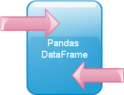 DataFrames live in system memory during execution; they do not permanently store data. To build automated data pipelines, you read data from external sources (spreadsheets, databases, files), transform it, and serialize the cleaned results back to disk or external databases.
Read our comprehensive guide to Data Input and Output from Pandas DataFrame →
1. Excel to MySQL Database Transfer
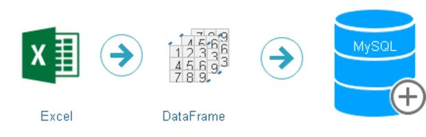
Read an Excel file (pd.read_excel()) and write directly into a relational MySQL database table using SQLAlchemy:
import pandas as pd
from sqlalchemy import create_engine

# 1. Read source records from Excel spreadsheet
df_emp = pd.read_excel("D:\emp.xlsx")

# 2. Establish connection to MySQL database via SQLAlchemy engine
# Connection string format: mysql+mysqldb://<user>:<password>@<host>/<dbname>
my_conn = create_engine("mysql+mysqldb://userid:password@localhost/database_name")

# 3. Create or append rows to the 'emp' table
df_emp.to_sql(con=my_conn, name="emp", if_exists="append", index=False)
print(f"Migrated {len(df_emp)} records from Excel to MySQL 'emp' table.")
2. MySQL Query to Excel Export
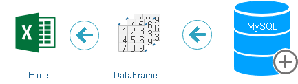
Execute an arbitrary SQL query against MySQL and export the resulting DataFrame into an Excel file for business distribution:
import pandas as pd
from sqlalchemy import create_engine

# 1. Connect to MySQL database
my_conn = create_engine("mysql+mysqldb://userid:password@localhost/database_name")

# 2. Query relational database directly into DataFrame
sql_query = "SELECT * FROM emp WHERE department = 'IT'"
df_it_staff = pd.read_sql(sql_query, con=my_conn)

# 3. Export to Excel workbook
df_it_staff.to_excel("D:\emp_it_report.xlsx", index=False)
print(f"Exported {len(df_it_staff)} records to emp_it_report.xlsx.")
Filtering Records & Axis Indexing 🔝
Pandas provides both label-based and boolean indexing to isolate target subsets of rows and columns:
| Feature | Description | Guide Link |
|---|---|---|
loc[] & iloc[] | Values at specific positions using column labels or integer positions | loc & iloc Selection → |
rows | Filtering rows based on conditional boolean logic and comparison masks | Row Filtering → |
String Manipulation with the str Accessor 🔝
The .str accessor provides vectorized text processing across text Series columns without explicit Python loops:
| String Function | Description | Detailed Tutorial |
|---|---|---|
str.contains() | Substring and pattern matching against text columns | str.contains → |
str.contains().sum() | Count matching rows meeting text criteria | str.contains.sum → |
str.lower() / str.upper() | Convert text case across column elements | Convert Case → |
str.split() | Break strings into lists using delimiters | split() → |
str.slice() | Extract substrings by start and stop character indices | slice() → |
str.cat() | Concatenate text from multiple columns or arrays | cat() → |
str.count() | Count regex pattern occurrences per row | count() → |
str.replace() | Replace text substrings using regex or literals | replace() → |
str.len() | Compute character length of text elements | len() → |
str.zfill() | Prepend zero padding to fixed string widths | zfill() → |
Data Visualization & Plotting 🔝
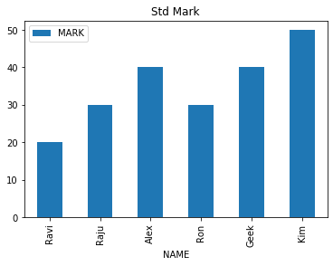
Visualizing DataFrames with Built-in Plotting
Pandas wraps Matplotlib directly through the df.plot() API, allowing you to generate line charts, bar charts, scatter plots, histograms, and box plots with a single command.
Column & Row Schema Operations 🔝
Shape, rename, and reorganize DataFrame schemas with dedicated column methods:
| Operation | Purpose & Behavior | Tutorial Link |
|---|---|---|
columns | Inspect, assign, or convert column headers | DataFrame Columns → |
rename() | Rename specific column labels or indices via mapping | Rename Columns → |
add_suffix() | Append a string suffix to all column names | add_suffix → |
add_prefix() | Prepend a string prefix to all column names | add_prefix → |
drop() | Remove unwanted columns or rows along axis 0 or 1 | drop() Columns/Rows → |
Pandas Namespace Introspection & Common Parameters 🔝
You can discover all available functions, classes, and sub-modules in the Pandas namespace using Python's built-in dir() function:
import pandas as pd

# 1. Total top-level functions and classes in pandas
pd_attributes = dir(pd)
print("Total attributes in pandas:", len(pd_attributes))

# 2. Inspect first 10 attributes
print(pd_attributes[:10])
Output:
Total attributes in pandas: 139
['BooleanDtype', 'Categorical', 'CategoricalDtype', 'CategoricalIndex', 'DataFrame', 'DateOffset', 'DatetimeIndex', 'DatetimeTZDtype', 'ExcelFile', 'ExcelWriter']
Understanding the inplace Parameter
Many Pandas transformation methods accept the inplace parameter:
| Parameter | Type | Default | Behavior |
|---|---|---|---|
inplace |
Boolean | False |
When set to True, the operation mutates the source DataFrame directly and returns None. When False (recommended in modern Pandas), a modified copy is returned, leaving the original intact. |
Cloud Data Access with Google Drive & Colab 🔝
Working on cloud notebooks like Google Colab allows you to ingest spreadsheets and CSVs directly from Google Drive:
Video Tutorial: Mount Google Drive and Load Files in Google Colab
Mount Drive syntax:from google.colab import drive; drive.mount('/content/drive')
Desktop GUI Integration with Tkinter 🔝
Integrating Pandas with Python's Tkinter library enables standalone desktop applications capable of importing spreadsheets, performing automated data cleaning, and rendering interactive tabular views and charts.
Explore Projects using Tkinter →Download Video Tutorial Project Files 🔝
Download the companion source code and reference files for this introductory tutorial module:
| Module | Description | Download Link |
|---|---|---|
| Section A | Pandas Introduction & Starter Scripts | 💾 Download ZIP |
Hands-on Starter Exercise: Departmental Analytics 🔝
Write a Python script that builds an employee DataFrame with 5 staff records across columns ["emp_id", "name", "department", "salary"]. Calculate the average salary for each department and filter all employees earning above $70,000.
import pandas as pd

employee_records = {
    "emp_id": [101, 102, 103, 104, 105],
    "name": ["Asha", "John", "Meera", "David", "Karan"],
    "department": ["IT", "Sales", "IT", "HR", "Sales"],
    "salary": [75000, 62000, 84000, 58000, 71000]
}

df_staff = pd.DataFrame(employee_records)

# 1. Average salary by department
dept_avg = df_staff.groupby("department")["salary"].mean().round(2)
print("Department Average Salaries:
", dept_avg)

# 2. Filter employees with salary > 70,000
high_earners = df_staff[df_staff["salary"] > 70000]
print("
High Earners (Salary > $70,000):
", high_earners[["name", "department", "salary"]])

# Self-checking assertions
assert len(high_earners) == 3
assert dept_avg["IT"] == 79500.00
assert "Meera" in high_earners["name"].values
print("
All unit assertions passed successfully!")
Interactive Practice in Google Colab & GitHub 🔝
Open in Google Colab View on GitHub
Experiment with Pandas Series, DataFrames, diagnostic tools, and departmental analytics interactively in Google Colab.
More Details & Related Guides 🔝
- Pandas DataFrame Guide — In-depth architectural guide to two-dimensional tabular data.
- Sample Student Dataset — Benchmark 35-row dataset used across all tutorial examples.
- Data Ingestion & I/O Hub — Connect Pandas to CSV, Excel, MySQL, SQLite, and JSON.
- Data Cleaning Hub — Comprehensive guide to handling nulls, duplicates, and invalid records.
- Data Analysis Hub — Exploratory data analysis, grouping, and aggregations.
- Data Visualization Hub — Complete guide to charting with Pandas and Matplotlib.
- Datetime & Time-Series Hub — Timestamps, periods, date offsets, and resampling.
- Pandas Real-World Projects — End-to-end case studies and production workflows.
- SEO Keyword Analytics — Text mining and search performance analysis with Pandas.

Subhendu Mohapatra
Author & Instructor at plus2net
I write and maintain practical tutorials on Python, PHP, SQL, JavaScript, HTML, jQuery, and web development at plus2net. The tutorials focus on clear explanations, working examples, and code that readers can test and adapt while learning.


Subscribe to our YouTube Channel here

 Python Video Tutorials