Pytrends
";require "templates/body_start.php";?>Pytrends is the unoffical API for Google Trends.If Pytrends is not installed, this error message will be displayed.
ModuleNotFoundError: No module named 'pytrends'
How to install Pytrend? In your command prompt enter this line.
pip install pytrendsInstalling Pytrend in Colab
!pip install pytrendsGetting today's trending search using trending_searches()
from pytrends.request import TrendReqpytrends = TrendReq()df = pytrends.trending_searches(pn='india')print(df)0 AHMEDABAD1 Putin2 Shani Jayanti 20223 Today news4 Nottingham Forest5 IP6 Legendrealtime_trending_searches()
We can usepn='US' , pn='IN' etc. for country specific search. List of countries with code is available here. df = pytrends.realtime_trending_searches(pn='CA')Top searches for the past years
We won't get data for the current year.df = pytrends.top_charts(2021, hl='en-US', tz=330, geo='IN')print(df)hl: Host Language. List of language codes are here. tz: Time zone. geo : Default value is GLOBAL, Other values are US ( USA) , FR (France), IN ( india ) , CA( Canada ), GB ( United Kingdom). Full List of countries with code is available heresuggestions
By using key word we can get suggestions from google trend.my_list=pytrends.suggestions('Digital Marketing') for val in my_list: print(val['type'],'->',val['title'])Related queries
kw=['Digital Marketing','Social media marketing','content marketing']pytrends.build_payload(kw_list=kw,timeframe='today 1-m',geo='IN')pytrends.related_queries()Managing time frame:
today 1-m : From today previous one month. Here month can only take values 1,3 or 12 only. now 1-d : Last one day only, it can take value 1 or 7 only. now 1-H : Last one hour, it works for 1 and 4 hours only. today 5-y : From today last 5 years '2021-12-19 2022-01-10' YYYY-MM-DD YYYY-MM-DD for specific period. '2022-02-06T10 2022-02-12T07' With datetime using UTC Related Topics
pytrends.build_payload(kw_list=['Digital Marketing'])df=pytrends.related_topics()df.values()Interest by region
kw=['Digital Marketing','Social media marketing','content marketing']pytrends.build_payload(kw_list=kw,timeframe='today 5-y',geo='IN')#pytrends.build_payload(kw_list=kw,timeframe='2022-02-06T10 2022-02-12T07',geo='US')pytrends.interest_by_region() Historical Hourly Interest
kw=['Python','PHP','JavaScript','HTML','MySQL']df=pytrends.get_historical_interest(kw, year_start=2020, month_start=1, day_start=1, hour_start=0, year_end=2020, month_end=2, day_end=1, hour_end=0, cat=0, geo='', gprop='', sleep=0)#df.plot(subplots=True, figsize=(20, 12)) date Python PHP JavaScript HTML MySQL isPartial0 2020-01-01 00:00:00 32 17 8 13 4 False1 2020-01-01 01:00:00 31 15 8 14 5 False2 2020-01-01 02:00:00 30 18 8 8 6 False3 2020-01-01 03:00:00 33 22 7 12 4 False4 2020-01-01 04:00:00 33 21 10 15 6 Falseimport pandas as pdkw=['Python','PHP','JavaScript','HTML','MySQL']df=pytrends.get_historical_interest(kw, year_start=2020, month_start=1, day_start=1, year_end=2021, month_end=1, day_end=10, cat=0, geo='', gprop='', sleep=0).reset_index()#print(df.columns)df['date']=pd.to_datetime(df['date'])df=df.resample('M', on='date').mean()print(df) Python PHP JavaScript HTML MySQL isPartialdate 2020-01-31 57.078877 27.098930 21.644385 27.423797 11.402406 0.02020-02-29 63.112857 27.844286 23.637143 30.468571 12.457143 0.02020-03-31 65.108289 28.981283 24.279412 31.517380 12.831551 0.02020-04-30 74.303448 29.267586 26.544828 33.942069 13.335172 0.02020-05-31 70.735294 28.426471 25.195187 32.414439 12.677807 0.02020-06-30 68.388122 29.237569 25.604972 31.824586 12.969613 0.02020-07-31 67.160214 28.958611 25.068091 30.510013 12.595461 0.02020-08-31 64.627005 27.794118 23.929144 29.491979 11.782086 0.02020-09-30 64.201379 25.779310 22.740690 29.801379 11.307586 0.02020-10-31 64.545455 25.631016 21.600267 29.926471 10.553476 0.02020-11-30 67.218232 27.556630 21.798343 30.788674 11.160221 0.02020-12-31 64.389853 27.753004 21.587450 29.837116 10.712951 0.02021-01-31 60.399083 27.871560 19.917431 27.233945 9.545872 0.0import pandas as pdkw=['Python','PHP','JavaScript','HTML','MySQL']df=pytrends.get_historical_interest(kw, year_start=2020, month_start=1, day_start=1, year_end=2021, month_end=1, day_end=10, cat=0, geo='', gprop='', sleep=0).reset_index()df['date']=pd.to_datetime(df['date']) # create date column df=df.resample('M', on='date').mean() # resample using monthly averagedf.reset_index(inplace=True) # remove index from date columndf.drop(labels='isPartial',axis=1,inplace=True) # delete coloumnprint(df.columns)df.plot(figsize=(10,5),x='date')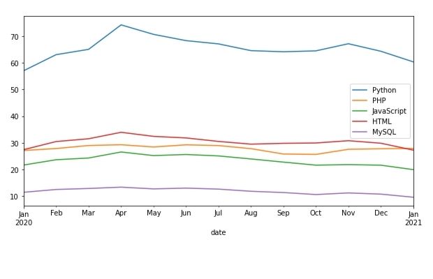
Note that numbers ( in Y Axis ) are scaled on a range of 0 to 100 based on a topic’s proportion to all searches on all topics.
Creating CSV or Excel file
We can collect data and store in a csv ( comma separated values ) or store in Excel file.import pandas as pdfrom pytrends.request import TrendReqpytrends = TrendReq()kw=['Python','PHP','JavaScript','HTML','MySQL']df=pytrends.get_historical_interest(kw, year_start=2020, month_start=1, day_start=1, year_end=2021, month_end=1, day_end=10, cat=0, geo='', gprop='', sleep=0).reset_index()#df.to_excel('D:\my_data\my_trends.xlsx',index=False) # excel filedf.to_csv('D:\my_data\my_trends.csv',index=False) # csv fileStoring in Database
We can use to_sql() to store data in MySQL Database.from sqlalchemy import create_enginemy_conn = create_engine("mysql+mysqldb://userid:pw@localhost/my_db")df.to_sql(con=my_conn,name='trends',if_exists='append')