Pandas Pie Charts: Percentages, Labels and Sales Shares

DataFrame.plot.pie() displays values as shares of their plotted total. Learn the plotting options with a small student dataset, then build a category revenue chart with a clear denominator. Choose a pie only when the values form meaningful parts of a whole.

Watch the demonstration, then run the notebook examples to compare labels, percentages and layout options.

Create a Pie Chart from One Numeric Column 🔝

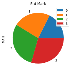
A pie shows each value as a share of the sum of the plotted values. Supply y="MATH" to select the numeric column. Without explicit labels or a named index, the slices use row labels. This small student example demonstrates the API; the sales example below gives a more natural part-of-whole use.

import pandas as pd
import matplotlib.pyplot as plt

def student_data():
    return pd.DataFrame({"NAME": ["Ravi", "Raju", "Alex", "Ronn"],
                         "MATH": [30, 40, 50, 50]})

df = student_data()
ax = df.plot.pie(y="MATH", title="Share of recorded MATH marks",
                 figsize=(5, 5), legend=False)
plt.tight_layout()
plt.show()
assert df["MATH"].sum() == 170

What to check: The denominator is 170 recorded marks, not a maximum possible exam score.

Choose Figure Size and Font Size 🔝

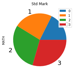
figsize is a width-height pair in inches. Equal dimensions work well for a circular chart. fontsize controls the category-label text; percentage text can also be adjusted through textprops. Increase the figure size before making already crowded labels larger.

df = student_data()
ax = df.plot.pie(y="MATH", title="Recorded marks", figsize=(4, 4),
                 fontsize=12, labels=df["NAME"].tolist(), legend=False)
plt.tight_layout()
plt.show()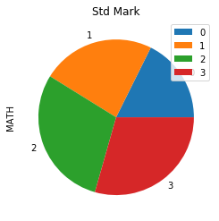

Use Category Names as Labels 🔝

A labels list must match the plotted values in length and order. Build it from the same DataFrame after any sorting or filtering. Alternatively, put the names in the index with set_index(). Keep category names short enough to read.

df = student_data()
my_labels = df["NAME"].tolist()
ax = df.plot.pie(y="MATH", labels=my_labels, fontsize=12,
                 title="Recorded marks by student", legend=False)
plt.tight_layout()
plt.show()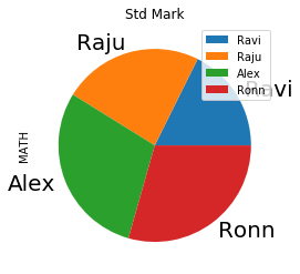

Control Label Distance and the Legend 🔝

labeldistance places labels at a fraction of the radius; 1.1 is outside the pie. You can suppress slice labels and use a legend with labeldistance=None. A legend is useful for longer category names, but readers still need clear colours and a small number of categories.

df = student_data().set_index("NAME")
ax = df.plot.pie(y="MATH", labeldistance=None, legend=True,
                 figsize=(6, 5), title="Recorded marks by student")
ax.legend(title="Student", loc="center left", bbox_to_anchor=(1, 0.5))
ax.set_ylabel("")
plt.tight_layout()
plt.show()

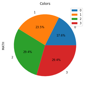
autopct: Display Each Share as a Percentage 🔝

autopct="%1.1f%%" displays one decimal place; %1.2f%% displays two. Percentages are calculated from the plotted sum. Rounded labels may not add to exactly 100%. Do not interpret a student's share of total marks as their exam percentage.

df = student_data().set_index("NAME")
ax = df.plot.pie(y="MATH", autopct="%1.1f%%", legend=False,
                 figsize=(5, 5), title="Share of recorded marks")
ax.set_ylabel("")
plt.tight_layout()
plt.show()
print((df["MATH"] / df["MATH"].sum() * 100).round(1))

Expected output

NAME
Ravi    17.6
Raju    23.5
Alex    29.4
Ronn    29.4
Name: MATH, dtype: float64

What to check: Ravi 17.6%, Raju 23.5%, Alex 29.4% and Ronn 29.4%.

Assign Colours in the Same Order as the Slices 🔝

The pie option is colors. Supply one colour per category for a predictable mapping. Use named colours or hexadecimal values. If you sort the values, rebuild the colour list from the category names so the same category keeps its colour.

df = student_data().set_index("NAME")
my_colors = ["lightblue", "lightgreen", "silver", "green"]
ax = df.plot.pie(y="MATH", colors=my_colors, legend=False,
                 autopct="%1.1f%%", figsize=(5, 5), title="Recorded marks")
ax.set_ylabel("")
plt.tight_layout()
plt.show()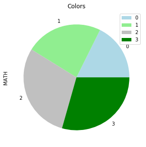

Highlight a Slice with explode 🔝

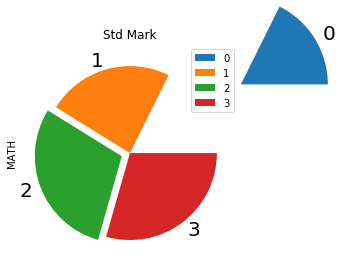
Each explode entry specifies the offset of a slice as a fraction of the radius. The tuple must have one entry per slice. Small offsets draw attention without disrupting the comparison. Very large offsets such as 1.5 separate a slice by more than a radius and make the chart harder to read.

df = student_data().set_index("NAME")
my_explode = (0, 0, 0.1, 0)
ax = df.plot.pie(y="MATH", explode=my_explode, legend=False,
                 figsize=(5, 5), title="Highlight Alex")
ax.set_ylabel("")
plt.tight_layout()
plt.show()

# Compare a deliberately large offset to understand the option.
ax = df.plot.pie(y="MATH", explode=(1.5, 0, 0.1, 0), legend=False,
                 figsize=(5, 5), title="Large offsets reduce readability")
plt.tight_layout()
plt.show()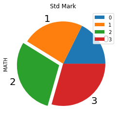

Set startangle and Drawing Direction 🔝

startangle rotates the first slice from the positive horizontal axis. counterclock=True draws in the default counterclockwise direction; False draws clockwise. These options change arrangement, not the values or percentages.

df = student_data().set_index("NAME")
ax = df.plot.pie(y="MATH", startangle=40, counterclock=False,
                 legend=False, figsize=(5, 5), title="Clockwise from 40 degrees")
ax.set_ylabel("")
plt.tight_layout()
plt.show()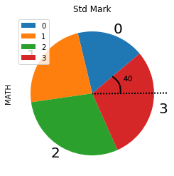

rotatelabels, shadow and frame 🔝

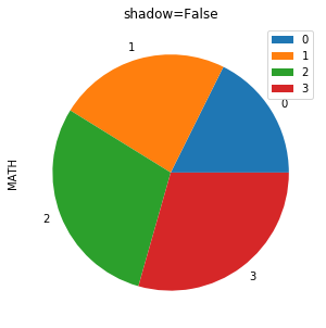
rotatelabels=True rotates category text with the slice direction; it can make labels harder to read. shadow=True adds a shadow, while frame=True shows the axes frame. A simple flat chart without rotated labels is usually easier to read. The example demonstrates all three controls so you can compare them.

df = student_data().set_index("NAME")
ax = df.plot.pie(y="MATH", rotatelabels=True, shadow=True, frame=True,
                 legend=False, figsize=(5, 5), title="Appearance options")
plt.tight_layout()
plt.show()

ax = df.plot.pie(y="MATH", rotatelabels=False, shadow=False, frame=False,
                 legend=False, figsize=(5, 5), title="Simple flat chart")
ax.set_ylabel("")
plt.tight_layout()
plt.show()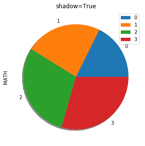

Practical Sales Example: Summarise Categories First 🔝

Pandas plots one slice per row, so repeated categories should be grouped before plotting. This synthetic dataset uses the same sales values as the bar-chart tutorial. The category totals are parts of one recorded revenue total and use the same units.

def sales_data():
    return pd.DataFrame({
        "category": ["Stationery", "Office", "Books", "Stationery", "Office", "Books"],
        "channel": ["Online", "Online", "Online", "Store", "Store", "Store"],
        "revenue": [120, 300, 180, 80, 250, 220]
    })

sales = sales_data()
totals = sales.groupby("category")["revenue"].sum().sort_values(ascending=False)
report = totals.to_frame("revenue")
report["share_percent"] = totals.div(totals.sum()).mul(100).round(1)
print(report)
assert totals.sum() == 1150
assert totals.to_dict() == {"Office": 550, "Books": 400, "Stationery": 200}

Expected output

            revenue  share_percent
category                          
Office          550           47.8
Books           400           34.8
Stationery      200           17.4

Plot Category Shares with a Clear Denominator 🔝

The title states that the pie represents recorded revenue. A supporting table provides exact amounts because similar-sized slices are hard to compare precisely. Use groupby() and sum() to prepare the totals, then plot the Series.

sales = sales_data()
totals = sales.groupby("category")["revenue"].sum().sort_values(ascending=False)
palette = {"Office": "#2563a6", "Books": "#df8b22", "Stationery": "#49845b"}
ax = totals.plot.pie(colors=[palette[name] for name in totals.index],
                      autopct="%1.1f%%", startangle=90, counterclock=False,
                      legend=False, figsize=(6, 5),
                      title="Share of recorded revenue (total 1,150)")
ax.set_ylabel("")
plt.tight_layout()
plt.show()

What to check: Office 47.8%, Books 34.8% and Stationery 17.4%. See the rendered chart in the notebook.

Validate Missing, Negative and Zero Values 🔝

A pie needs finite, non-negative values and a positive total. Unknown revenue must not silently become zero. Negative values, such as refunds, need a different report. Validate the plotted Series before charting; do not let an all-missing group become a zero total. For incomplete inputs, follow the missing-value guidance.

import numpy as np

def validate_pie_values(values):
    numeric = pd.to_numeric(values, errors="raise").astype("float64")
    if not np.isfinite(numeric.to_numpy()).all():
        raise ValueError("Pie values must be known and finite.")
    if numeric.lt(0).any():
        raise ValueError("Pie values cannot be negative.")
    if numeric.sum() <= 0:
        raise ValueError("Pie values need a positive total.")
    return numeric

for values in ([20, 30], [20, None], [20, -5], [0, 0]):
    try:
        checked = validate_pie_values(pd.Series(values))
        print("Valid total:", checked.sum())
    except ValueError as error:
        print(error)

Expected output

Valid total: 50.0
Pie values must be known and finite.
Pie values cannot be negative.
Pie values need a positive total.

Combine Small Categories Without Losing the Total 🔝

Too many slices make labels and proportions difficult to read. Combine smaller categories as Other under a stated rule, or use a horizontal bar chart. Here the two largest categories are kept individually; the remainder becomes Other. Check that the displayed total matches the original.

amounts = pd.Series({"Office": 550, "Books": 400, "Stationery": 200,
                     "Accessories": 60, "Other supplies": 40})
ordered = validate_pie_values(amounts).sort_values(ascending=False)
display = pd.concat([ordered.iloc[:2],
                     pd.Series({"Other": ordered.iloc[2:].sum()})])
print(display)
assert display.sum() == amounts.sum()
ax = display.plot.pie(autopct="%1.1f%%", legend=False, figsize=(5, 5),
                       title="Two largest categories; remainder as Other")
ax.set_ylabel("")
plt.tight_layout()
plt.show()

Expected output

Office    550.0
Books     400.0
Other     300.0
dtype: float64

Save Your Pie Chart as a PNG 🔝

Save the returned Axes figure before closing it. A relative filename works in Colab and on your computer. In Colab, download the file from the Files sidebar; saving in the runtime does not automatically copy it to Drive. See the Colab guide for file handling.

df = student_data().set_index("NAME")
ax = df.plot.pie(y="MATH", autopct="%1.1f%%", legend=False,
                 figsize=(5, 5), title="Share of recorded marks")
ax.set_ylabel("")
plt.tight_layout()
fig = ax.get_figure()
fig.savefig("pandas_pie_chart.png", dpi=150, bbox_inches="tight")
plt.show()
print("Saved pandas_pie_chart.png")

Expected output

Saved pandas_pie_chart.png

When a Bar Chart Is a Better Choice 🔝

Use a pie for a few mutually exclusive, non-negative parts of a meaningful whole. Use bars for exact category comparisons, similar values, negative values or multiple series. Use lines to show change over time. Do not put quantities, prices and revenue into one pie: their units do not form a common whole. Multiple pies each normalise to their own total, so they can hide large differences in size.

Exercise: Revenue Share by Channel 🔝

Group the sales data by channel and plot the Online and Store shares with one-decimal percentage labels. Predict the denominator and both percentages. Expected total: 1,150; Online 52.2%, Store 47.8%.

Exercise Solution 🔝

The channel totals are mutually exclusive parts of the same recorded revenue. Validate them before plotting, and check that the two totals add up to the source revenue.

sales = sales_data()
totals = validate_pie_values(sales.groupby("channel")["revenue"].sum())
print(totals)
print(totals.div(totals.sum()).mul(100).round(1))
assert totals.to_dict() == {"Online": 600, "Store": 550}
assert totals.sum() == sales["revenue"].sum()
ax = totals.plot.pie(autopct="%1.1f%%", startangle=90,
                      legend=False, figsize=(5, 5), title="Revenue share by channel")
ax.set_ylabel("")
plt.tight_layout()
plt.show()

Expected output

channel
Online    600.0
Store     550.0
Name: revenue, dtype: float64
channel
Online    52.2
Store     47.8
Name: revenue, dtype: float64

Practice in Google Colab 🔝

Open in Google Colab View on GitHub
All datasets and rendered example charts are included. Run the cells, adjust the options and try the exercise. Save a copy in Drive to keep your changes.

Continue with the Pandas Plot guide and plotting exercises. Explore box, density, area, scatter and hexbin plots for other questions.

Reference: Pandas pie-plot documentation.

Subhendu Mohapatra

Author & Instructor at plus2net

I write and maintain practical tutorials on Python, PHP, SQL, JavaScript, HTML, jQuery, and web development at plus2net. The tutorials focus on clear explanations, working examples, and code that readers can test and adapt while learning.

About the author   Watch on YouTube

Connect: